



Long Lead Time Components: Forecasting and Mitigation Strategies
Component lead times reached unprecedented levels in 2024-2025, with power management ICs, MCUs, and specialty passive components stretching to 40+ weeks. While the acute shortage has eased slightly in 2026, procurement teams still face a bifurcated market: commodity parts ship within days, but application-specific controllers, automotive-grade power devices, and mature-node analog ICs remain constrained. For engineers and procurement managers, long lead times translate directly to production delays, increased inventory costs, and lost revenue opportunities.
At Hitop Tech Limited, our procurement services help clients navigate extended lead times through demand forecasting, allocation management, and multi-source strategies that maintain production continuity even during supply constraints.
Table of Contents
- Understanding the Lead Time Problem in 2026
- Demand Forecasting Methods That Actually Work
- Allocation Management and Supplier Communication
- Buffer Stock Strategies and Inventory Optimization
- Alternative Component Sourcing and Design Flexibility
- Regional Lead Time Differences and Split Allocation
- FAQ
- Conclusion
1. Understanding the Lead Time Problem in 2026
Lead times vary dramatically by component category and manufacturing node. While cutting-edge 3nm and 5nm process technology receives heavy investment and new fab capacity, mature nodes (28nm to 180nm) that produce the bulk of automotive MCUs, power management ICs, analog devices, and discretes remain capacity-constrained.
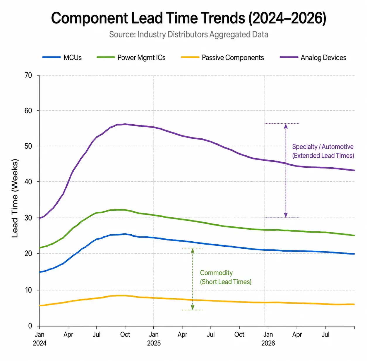 Component lead time trends by category showing bifurcation between commodity and specialty parts in 2026
The table below shows current lead time ranges by component category as of Q2 2026, based on data from authorized distributors and direct manufacturer quotes:
| Component Category | Standard Lead Time (weeks) | Extended Lead Time (weeks) | Primary Constraint Factor |
|---|---|---|---|
| Standard MCUs (general purpose) | 8-12 | 16-24 | Wafer allocation |
| Automotive MCUs (AEC-Q100) | 26-32 | 38-52 | Qualification + capacity |
| Power Management ICs (high current) | 16-20 | 28-40 | Substrate + packaging |
| Low-Dropout Regulators (automotive) | 12-18 | 24-32 | Testing capacity |
| MOSFETs (>100V, automotive) | 14-22 | 30-45 | Wafer starts |
| Specialty MLCCs (high voltage) | 10-16 | 20-30 | Dielectric layer process |
| Crystal Oscillators (custom freq) | 8-12 | 18-26 | Custom manufacturing |
| Analog Front-Ends (medical grade) | 18-26 | 36-48 | Qualification + yield |
The bifurcation is stark. Commodity resistors, ceramic capacitors in standard ratings, and jellybean transistors ship within 2-6 weeks. Application-specific standard products (ASSPs), automotive-qualified devices, and anything requiring custom parameters or extended temperature ranges face dramatically longer queues. Understanding where your critical components fall on this spectrum determines which mitigation strategies will be most effective.
2. Demand Forecasting Methods That Actually Work
Accurate forecasting directly reduces inventory costs and stockout risk. The methods below, used in combination, improve forecast accuracy by 30-45% compared to single-method approaches.
Rolling Forecast with Demand Sensing
Implement a 52-week rolling forecast updated monthly, with the first 12 weeks locked as firm commitments and weeks 13-26 as flexible forecast. Use point-of-sale data, production schedule visibility, and design-win pipeline to sense demand shifts early.
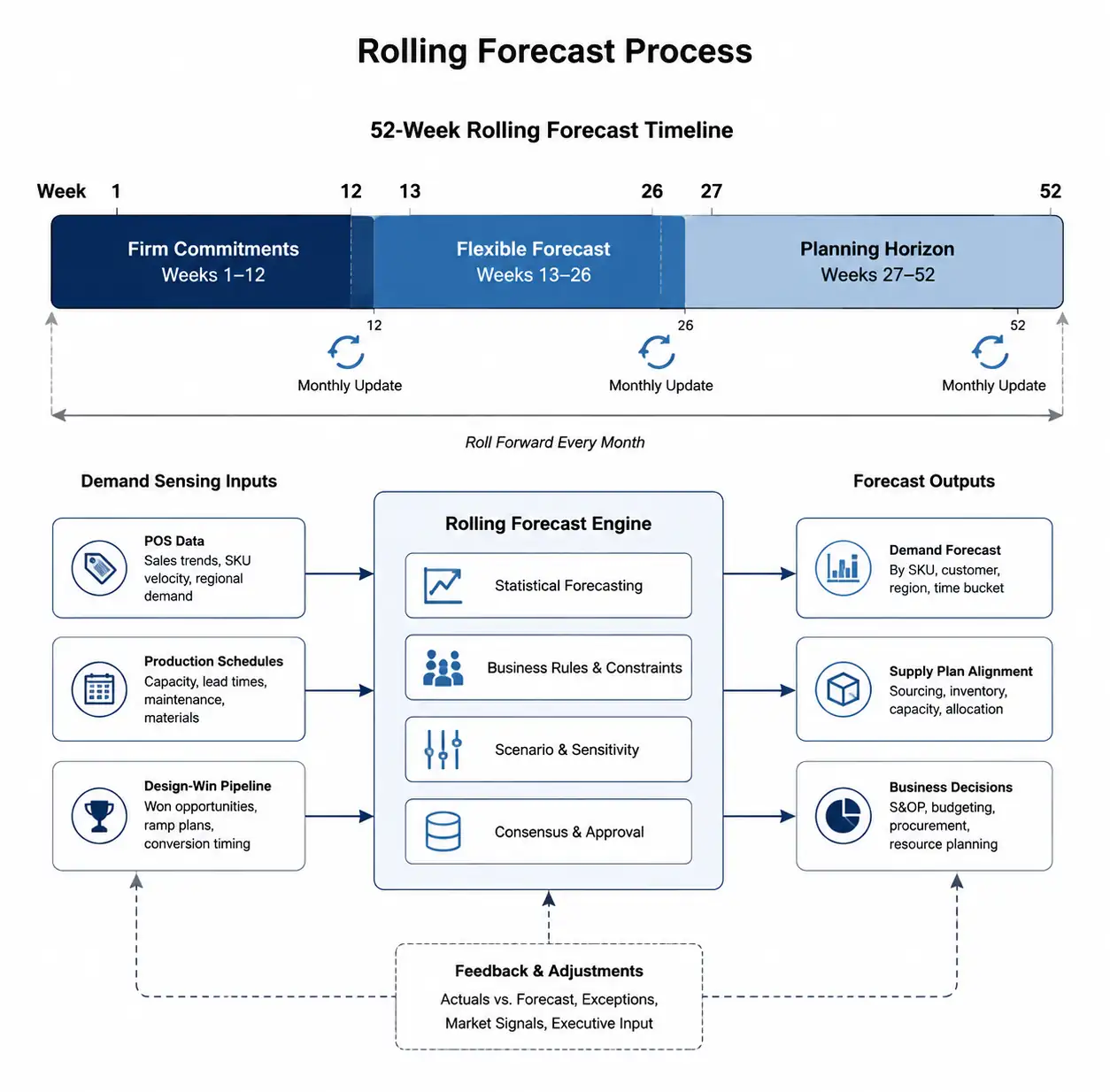 Rolling 52-week demand forecast workflow diagram with firm commitment and flexible forecast zones
Safety Stock Calculation for Long Lead Times
Calculate safety stock using: Safety Stock = Z × σLT × √(LT), where Z is the service level factor (1.65 for 95% service level), σLT is demand standard deviation during lead time, and LT is lead time in weeks. For components with >26-week lead times, adjust Z upward to 1.96 (97.5% service level).
Track new product introductions separately from sustaining demand. Establish a design-win database capturing project name, production start date, volume ramp profile, and component list. Update probability-weighted forecasts monthly to prevent sudden demand spikes when prototypes transition to production.
| Forecasting Method | Best Application | Typical Accuracy Improvement | Update Frequency |
|---|---|---|---|
| Rolling 52-week forecast | High-volume products, stable demand | Baseline | Monthly |
| Demand sensing with POS data | Consumer electronics, seasonal products | +15-25% | Weekly |
| Consumption + safety stock | Industrial, automotive sustaining | +10-15% | Monthly |
| Design-in tracking | NPI, project-based demand | +25-40% for NPI | Bi-weekly |
| Hybrid statistical + judgment | Mixed product portfolio | +30-45% overall | Monthly core, weekly adjustments |
For components with lead times exceeding 26 weeks, forecast horizon should extend to at least 2× the lead time to place orders before stock depletes.
3. Allocation Management and Supplier Communication
When demand exceeds supply, manufacturers implement allocation—distributing available capacity based on historical purchases, strategic relationships, and forecast commitments. Effective allocation management requires proactive communication and clear commitment strategies.
Manufacturers typically allocate based on trailing 12-month (TTM) purchase history, with adjustments for strategic account status, long-term agreements (LTAs), and forecast accuracy. A customer who consistently orders 70% of forecasted quantities receives lower allocation priority than one who pulls 95%+ of commitments.
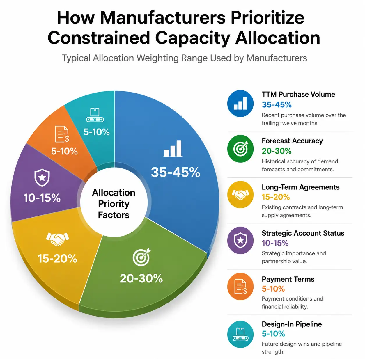 Manufacturer allocation priority factors showing weighted criteria for customer allocation decisions
To secure allocation during tight supply, be prepared to commit to NCNR (non-cancellable, non-returnable) terms for critical components. NCNR orders receive higher allocation priority because they represent firm demand. For automotive programs with multi-year production runs, NCNR commitments on 26+ week lead time components are standard practice.
When demand forecasts change, communicate immediately—even if it means reducing future pull. Suppliers remember which customers provide accurate, timely updates versus those who submit inflated forecasts. This transparency builds allocation goodwill that pays dividends when supply tightens again.
The table below shows allocation priority factors and their typical weighting in manufacturer allocation decisions:
| Allocation Priority Factor | Typical Weight | How to Improve Your Position |
|---|---|---|
| TTM purchase volume | 35-45% | Consolidate purchases, increase wallet share |
| Forecast accuracy (pull vs. commit) | 20-30% | Improve forecasting, commit conservatively |
| Long-term agreement in place | 15-20% | Negotiate 1-3 year LTA with volume commitments |
| Strategic account designation | 10-15% | Executive engagement, design-in activity |
| Payment terms and credit standing | 5-10% | Maintain net-30 or better, clean payment history |
| Design-in pipeline visibility | 5-10% | Share NPI roadmap, invite FAE engagement |
Suppliers allocate to customers they trust to pull forecast quantities and communicate changes transparently. If your organization has historically canceled orders or pushed deliveries repeatedly, allocation will reflect that behavior regardless of current need.
4. Buffer Stock Strategies and Inventory Optimization
Buffer stock protects against demand variability and supply disruptions, but excessive inventory ties up capital and risks obsolescence. The optimal buffer stock level balances service level targets against carrying costs.
For components with >20-week lead times, traditional EOQ formulas underestimate optimal order quantities. Use modified EOQ: Q* = √(2DS/H) × √(1 + (σLT²/LT²)), where D is annual demand, S is order cost, H is holding cost per unit per year, σLT is lead time standard deviation, and LT is average lead time.
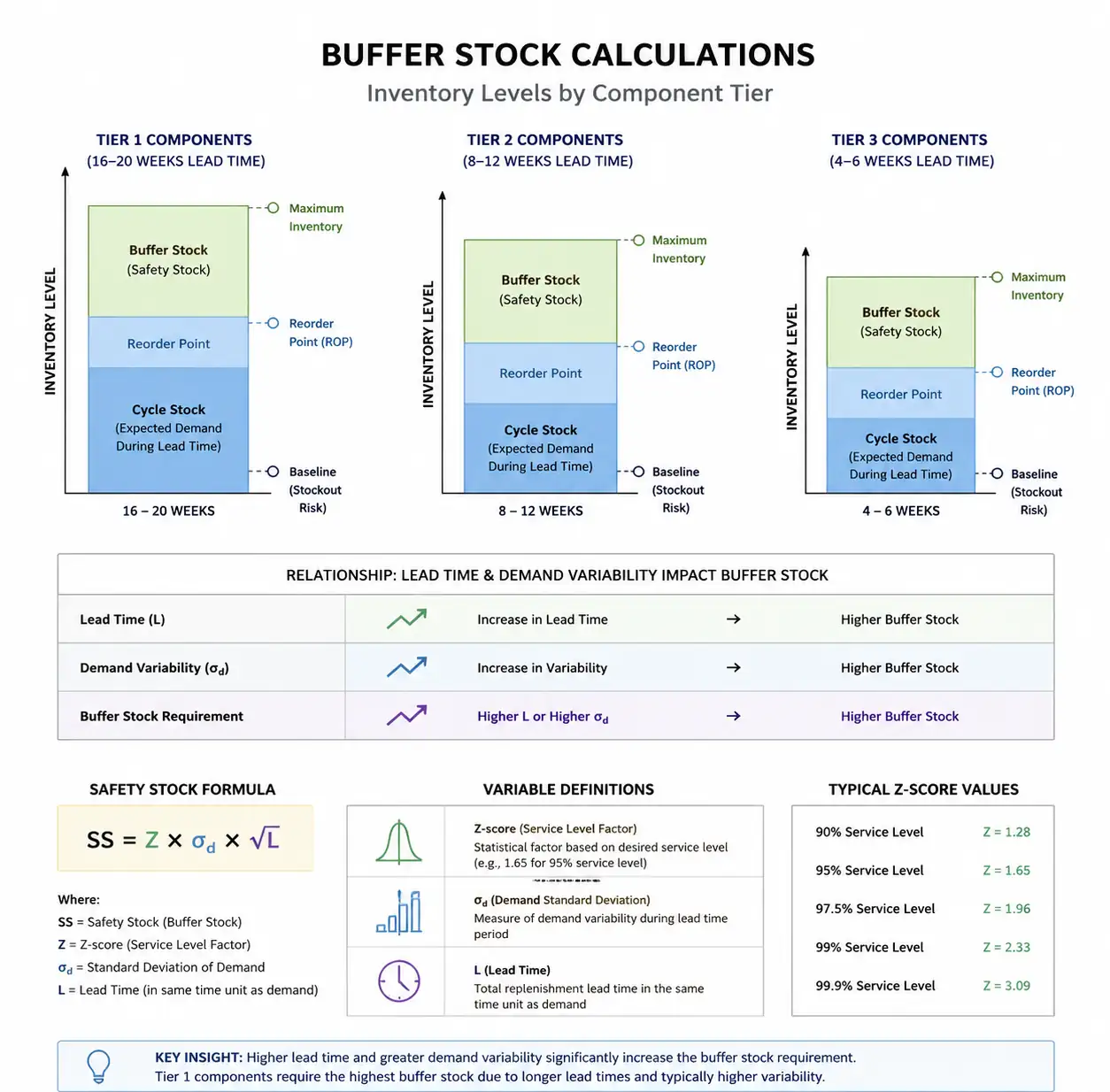 Buffer stock calculation diagram showing safety stock levels for different component lead time scenarios
Segment your BOM into three tiers: Tier 1 components are single-source, long lead time (>26 weeks), high production impact—maintain 16-20 weeks of buffer stock. Tier 2 components have alternative sources or moderate lead times (12-26 weeks)—maintain 8-12 weeks buffer. Tier 3 commodity components with <12-week lead times and multiple sources—maintain 4-6 weeks buffer.
For high-volume stable demand, negotiate VMI (vendor-managed inventory) or consignment arrangements where the supplier maintains buffer stock at your facility. You pay only upon consumption, shifting inventory carrying costs to the supplier.
When a manufacturer issues EOL (End-of-Life) announcement, calculate last-time-buy quantities based on remaining product lifetime plus service tail requirements. For automotive products with 10-15 year service obligations, EOL buffer stocks can represent multiple years of production.
5. Alternative Component Sourcing and Design Flexibility
The most effective mitigation strategy is eliminating single-source dependencies before they become crises. Alternative component sourcing requires upfront engineering investment but pays dividends when primary sources face constraints.
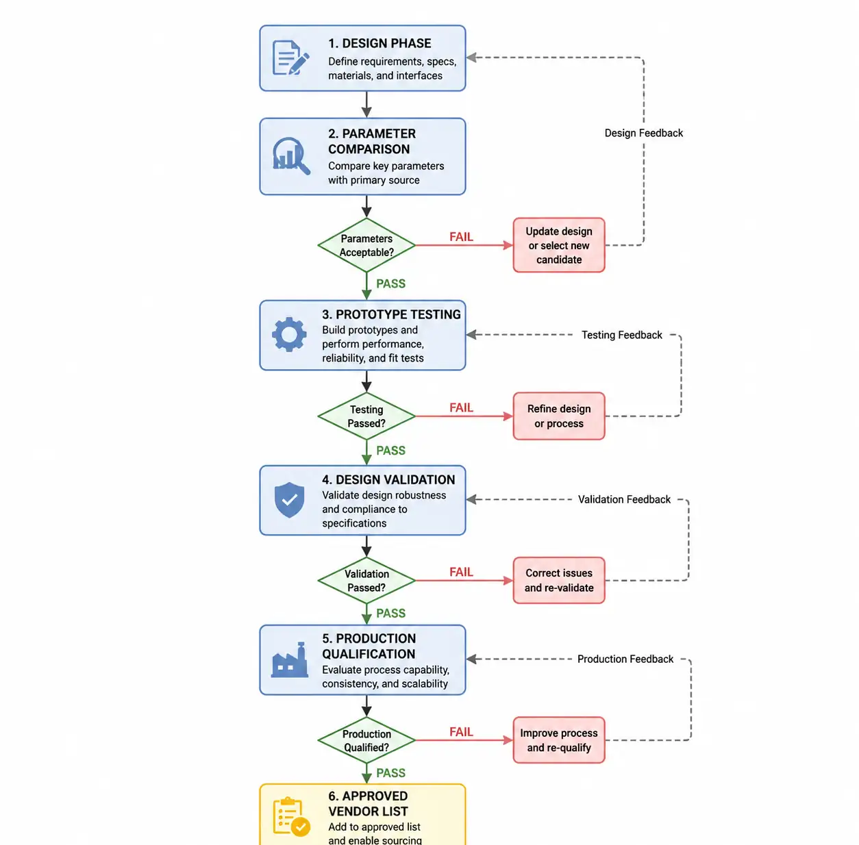 Second-source component qualification process flowchart from design phase through production approval
Qualifying alternative components during the design phase costs 10-20% more upfront but eliminates 80% of lead time risk. For critical power management, MCUs, and analog devices, design with pin-compatible alternatives from multiple manufacturers. Texas Instruments, Analog Devices, Maxim Integrated, and Microchip often have competing devices with similar specifications.
For industrial and commercial applications, form-fit-function (FFF) equivalents—parts with identical footprint, pinout, and specifications—can often be substituted with abbreviated verification testing. Document critical parameters that must match and parameters where variation is acceptable.
Incorporate design margin that accommodates parameter variation across alternative sources. If your power supply design requires <100µV output ripple, and alternative regulators range from 50-120µV, increase output filtering to guarantee <100µV across all sources. Adding $0.15 in capacitors eliminates $50K in re-qualification costs.
| Sourcing Strategy | Implementation Cost | Lead Time Risk Reduction | Best Application |
|---|---|---|---|
| Second-source qualification | Medium (10-20% NRE increase) | 70-85% | MCUs, power management, critical analog |
| Form-fit-function substitution | Low (5-10% testing cost) | 60-75% | Standard functions, industrial applications |
| Design margin for flexibility | Low (1-3% BOM cost) | 50-70% | Precision circuits with multiple sources |
| Modular design with interfaces | High (30-50% design time) | 85-95% | Complex subsystems, multi-generation products |
| Authorized distributor franchises | None | 30-40% | Broad commodity components |
Working with an experienced distributor like Hitop Tech Limited provides access to authorized franchise lines from multiple manufacturers, enabling quick pivots to alternative sources when primary suppliers face constraints.
6. Regional Lead Time Differences and Split Allocation
Component lead times vary significantly by region due to differences in fab capacity, distribution networks, and demand patterns. Strategic sourcing across regions can reduce effective lead times by 20-35%.
For power discretes, passive components, and connectors manufactured primarily in Asia, local procurement from Asian distributors typically delivers 2-4 weeks faster than ordering through North American or European distribution. If your production is in Southeast Asia, sourcing from Singapore, Taipei, or Hong Kong hubs reduces pipeline time.
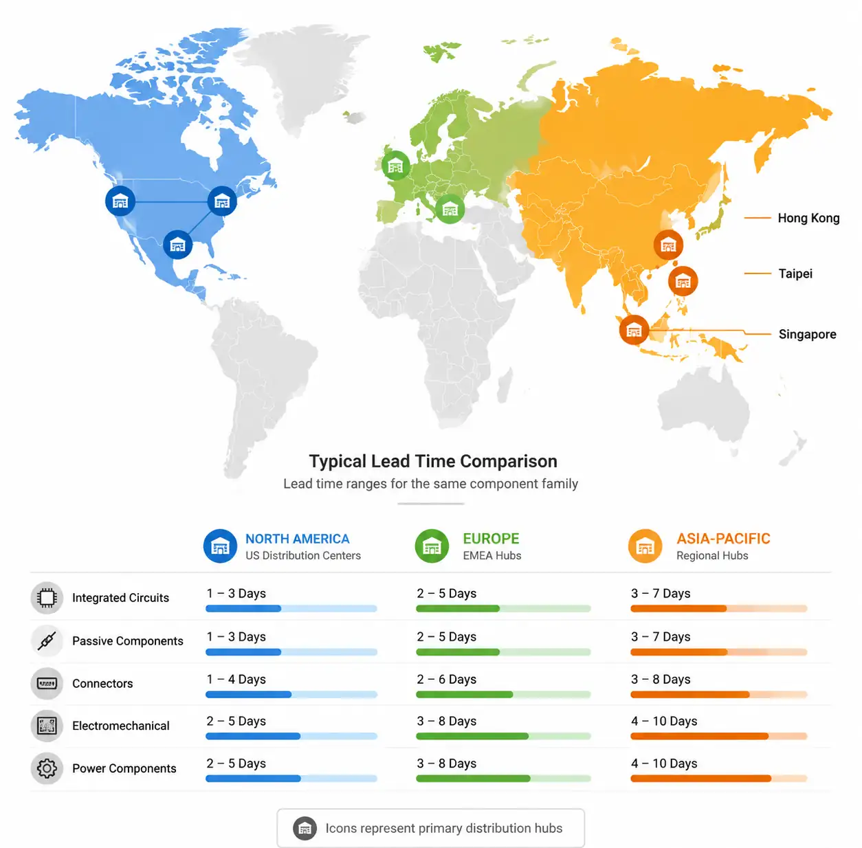 Global regional lead time comparison showing distribution hub advantages in Asia-Pacific, North America, and Europe
Global manufacturers maintain regional inventory buffers to serve local demand. During allocation periods, the Americas distribution center might show 12-week lead times while EMEA shows 20 weeks for the same part number. Split your allocation requests across regions—order 60% from your primary region and 40% from secondary regions with better availability.
Cross-border procurement adds complexity: import duties (0-5% for most components under HTS 8542), customs clearance (2-5 days), and compliance documentation (RoHS, REACH). Air freight from Asia to North America adds 3-7 days transit time. For buffer stock, ocean freight reduces logistics costs by 60-75% at the expense of 4-6 weeks transit.
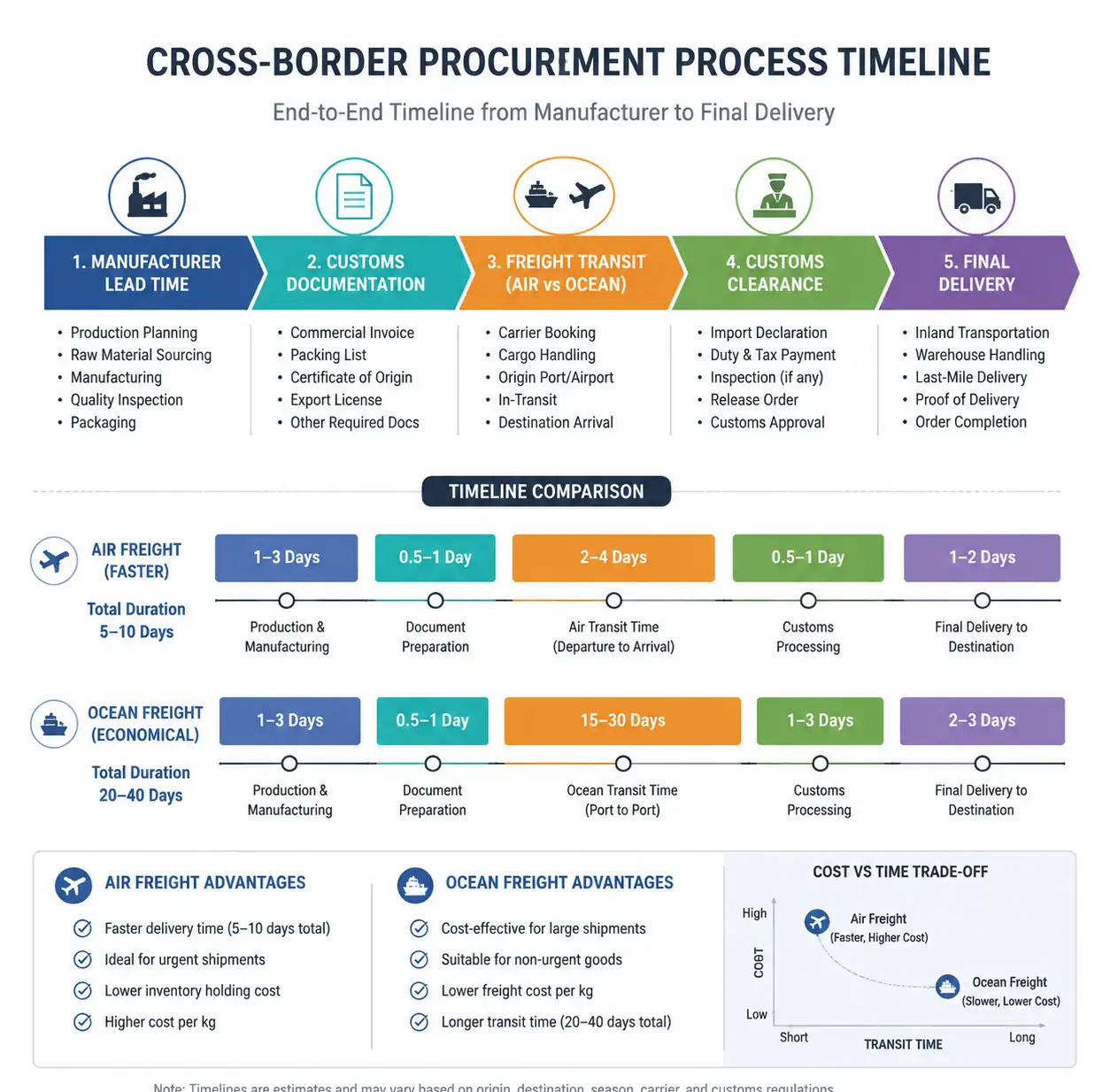 Cross-border component procurement timeline showing lead time, customs clearance, and freight transit phases
Our procurement services manage multi-region sourcing and logistics coordination, ensuring components arrive when needed while minimizing total acquisition cost.
7. FAQ
What is the difference between lead time and delivery time?
Lead time is the period from order placement to shipment from the manufacturer or distributor. Delivery time includes lead time plus transportation and customs clearance. For overseas orders, delivery time can be 1-6 weeks longer than quoted lead time depending on shipping method and customs.
How do I know if my forecast commitment is strong enough to secure allocation?
Compare your historical pull rate (actual orders / forecasted quantities) over the trailing 12 months. If you consistently pull 85% or more of your 3-month-out forecast, your commitment carries weight. Below 75% pull rate, expect lower allocation priority unless you negotiate an LTA with NCNR terms.
Should I hold buffer stock for all long lead time components?
No. Prioritize buffer stock for single-source components with >20-week lead times that are critical to production and have stable demand. For components with multiple qualified sources or volatile demand, better strategies are second-source qualification or vendor-managed inventory.
When should I issue a last-time-buy order for an EOL component?
Calculate your last-time-buy quantity as soon as EOL is announced: (remaining production life + service obligation) × annual consumption × 1.25 safety factor. Place orders immediately if the EOL notice gives <6 months to final order date. For automotive and medical devices with 10+ year service tails, coordinate with your product lifecycle team to balance inventory costs against redesign costs.
How can I reduce lead times without increasing costs?
Focus on forecast accuracy and transparent supplier communication. Suppliers allocate capacity to customers they trust. Improving your 6-month forecast accuracy from 60% to 85% can move you from standard to preferred allocation tier, effectively cutting lead times by 20-30% without increasing piece price.
What are the risks of ordering through brokers to avoid long lead times?
Broker-sourced components carry higher counterfeit risk, no manufacturer warranty, and uncertain traceability. For non-critical commercial applications, reputable brokers can fill gaps. For automotive, medical, aerospace, or safety-critical applications, broker sourcing is unacceptable—use authorized distribution or manufacturer direct only. See our guide on verifying component authenticity for more details.
How do regional tariffs affect component lead times and sourcing decisions?
Tariffs primarily affect cost, not lead time, but they can influence sourcing strategy. If a 15% tariff applies to imports from Region A but not Region B, sourcing from Region B makes economic sense even if lead time is 2 weeks longer. Evaluate total landed cost including tariffs, freight, and carrying cost, not just piece price and lead time.
8. Conclusion
Managing long lead time components requires a multi-layered approach combining accurate demand forecasting, transparent supplier relationships, strategic buffer stock, and design flexibility. The most successful procurement strategies don't rely on a single mitigation technique but instead deploy 3-4 complementary approaches tailored to component criticality and supply risk.
If your forecast accuracy is below 80%, improving forecasting delivers the highest return. If you're already forecasting well but facing allocation constraints, invest in supplier relationships through LTAs and communication transparency. For new designs, prioritize second-source qualification during development rather than scrambling for alternatives during production.
Long lead times will remain a structural challenge as long as mature-node fab capacity lags demand for automotive, industrial, and IoT applications. Procurement teams that treat lead time management as a core competency—not just a reactive firefight—will maintain production continuity and cost competitiveness through the next supply cycle.
For expert support navigating component lead times, allocation management, and multi-source strategies, contact Hitop Tech Limited. Request a quote for your next project, or explore our supplier consolidation services to streamline your supply chain.